Getting Launch Monitor Data into R
What this tutorial covers
As an analyst or data scientist, one thing they don’t tell you in school is how much time you’ll spend accessing, scraping, extracting, wrangling, munging, cleaning, transforming, shaping, prepping, and a hundred other verbs that all essentially mean “get the data into a form that allows us to cleanly analyze, visualize, or model.”
This kind of work tends to get abbreviated to three letters: ETL (or ELT), which stands for Extract, Transform, Load, and it’s exactly what we’re going to do here.
This first tutorial will cover:
- Exporting data from Foresight
- Installing R and R-Studio
- Loading the data into R and prepping it for analysis
Let’s get started!
STEP 1: Get Data
I expect you’ll eventually want to get your own data in here, but for the purposes of this tutorial I’ve provided an export of my data from a session on my GC3 comparing Driver and 3-Wood. If you don’t plan on using your own data just yet, you can download the .csv here and skip ahead to step 2.
If you have your own Foresight Launch Monitor or have access to one via a golf pro, fitter, or even your local golf superstore, I’m going to show you how to export a custom report that will look identical to my own. This way you hopefully won’t need to modify any of the code.
If you have a different kind of launch monitor (Trackman, Mevo+, etc…) and want to be able to analyze your data, feel free to email an export of your data to me at michaeldavidhutchinson@gmail.com and I can add some code to clean and work with it. Eventually I’d like to build a large database for different types of analysis, so if you have data, send it over.
Anyway, here’s how to export data with Foresight….
- From the Foresight range, click on the icon that looks like a side view of ball flight data.
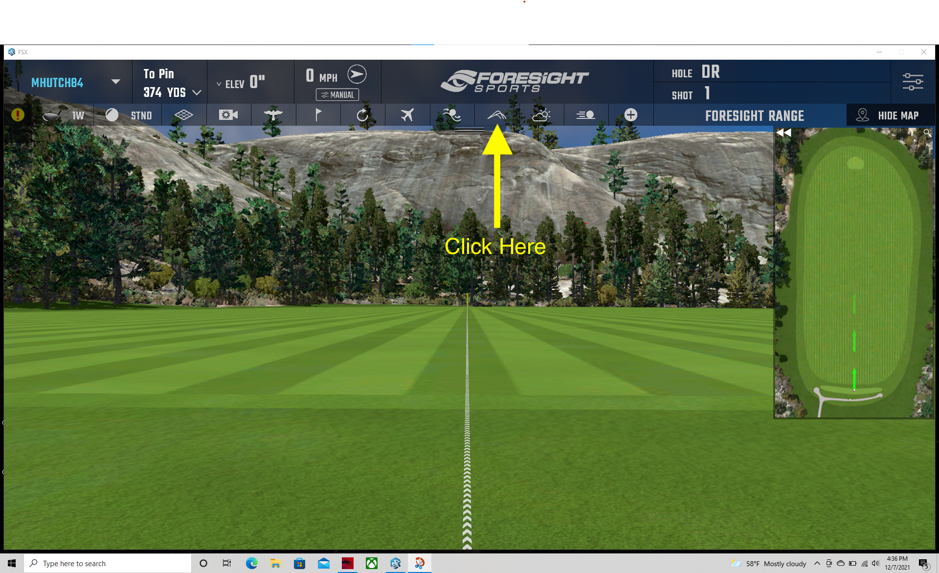
Figure 1: Foresight Range
- From this data view screen, click EXPORT in the top right corner.
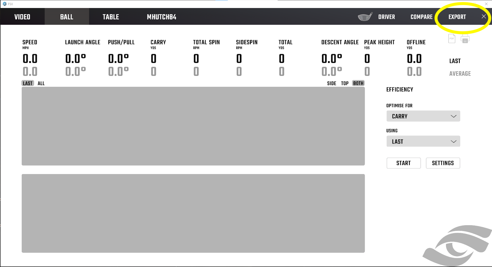
Figure 2: Data View
- In the report manager view, you’re going to create a custom report.

Figure 3: Report Manager View
- Select all available fields for ball and club data, regardless of whether your specific simulator captures the variable. This ensures consistency in the data across all reports so that the code runs as expected. It’s also nice to have a report that just captures everything. Give the report a name and hit Save/Add.
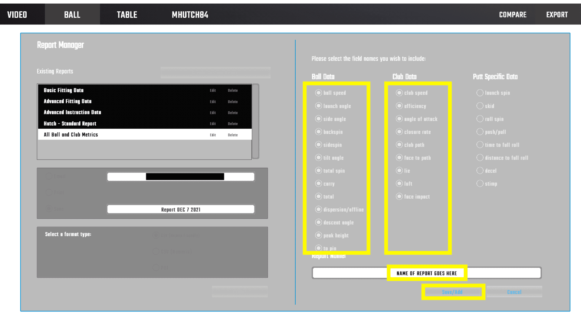
Figure 4: Custom Report
- The name of your custom report will now appear in the list of the standard reports. Choose the report (the white report is the one that is currently selected). You can email or save it locally as a .csv.
I have exported both the “Human Friendly” and “Numeric” .csv versions, and they each need some work to get into a tidy dataset, but the “Numeric” version is easier to work with.
Save the exported file somewhere you’ll be able to access it. We’ll move it to its final location in a little bit.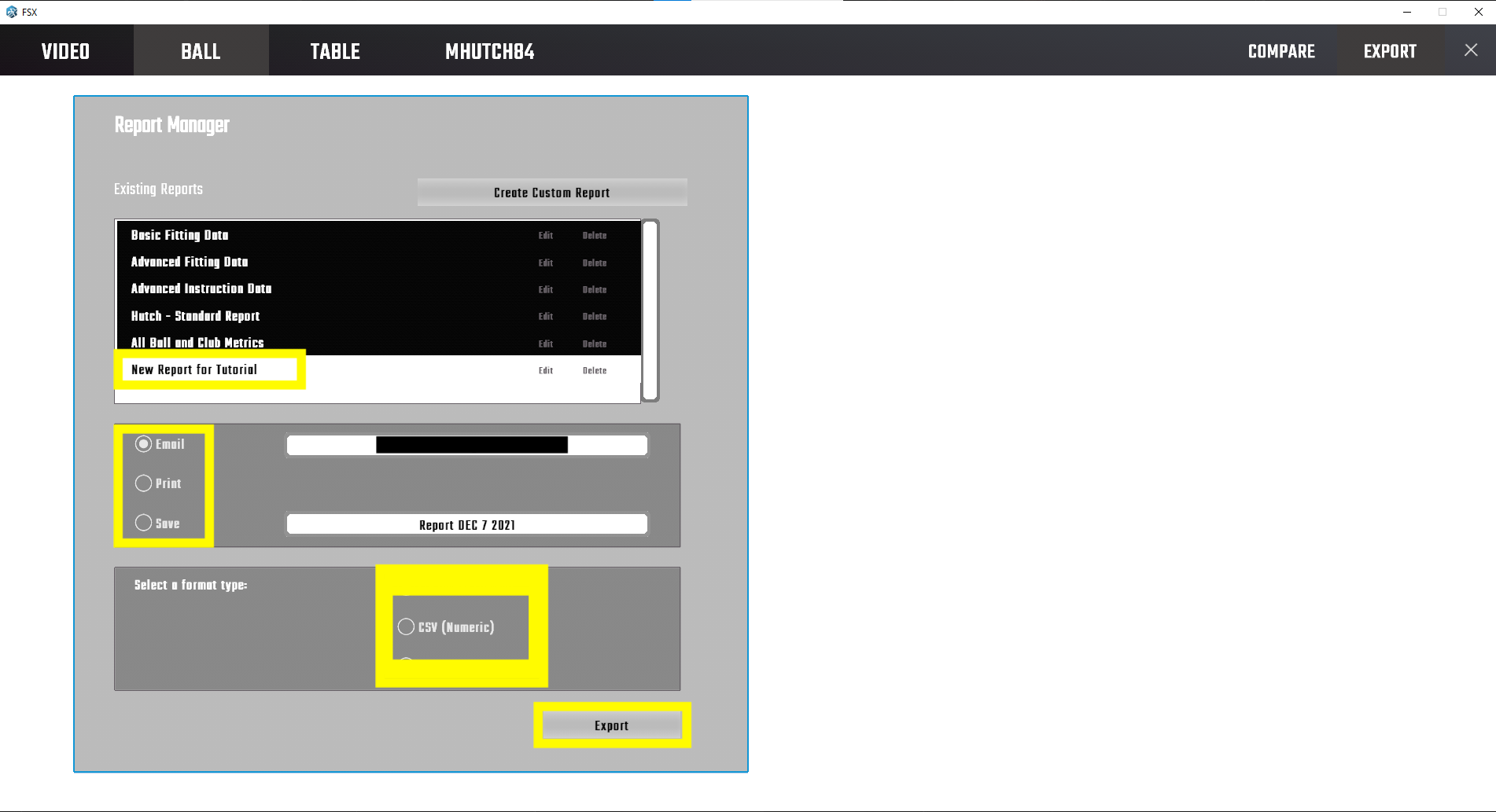
Figure 5: Custom Report
Okay! Save that file somewhere you’ll remember because we’re going to come back to it in a bit.
STEP 2: Install R
Assuming you don’t already have it installed, there are tons of great tutorials out there about how to get up and running with R and R Studio, so I won’t go into much detail here. This tutorial from Datacamp has everything you need to get started whether you’re on Mac, Windows, or Ubuntu. If that doesn’t work, a quick Google search will get you plenty of solid options.
STEP 3: Create New R Project
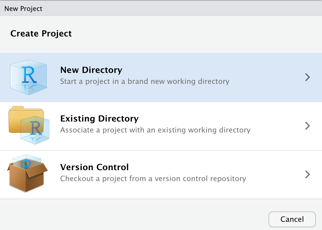
Now that we have R installed, let’s start by opening R Studio and creating a new project by going to: File -> New Project.
You don’t have to do these next steps exactly as I did, and the userflow may be slightly different depending on your OS and version, but it’s good practice to create self contained new projects with organized directories, and as I’m learning, that’s even more important if you want to build a website. Anyway, here’s what that looks like…
1. Create project in a new directory.
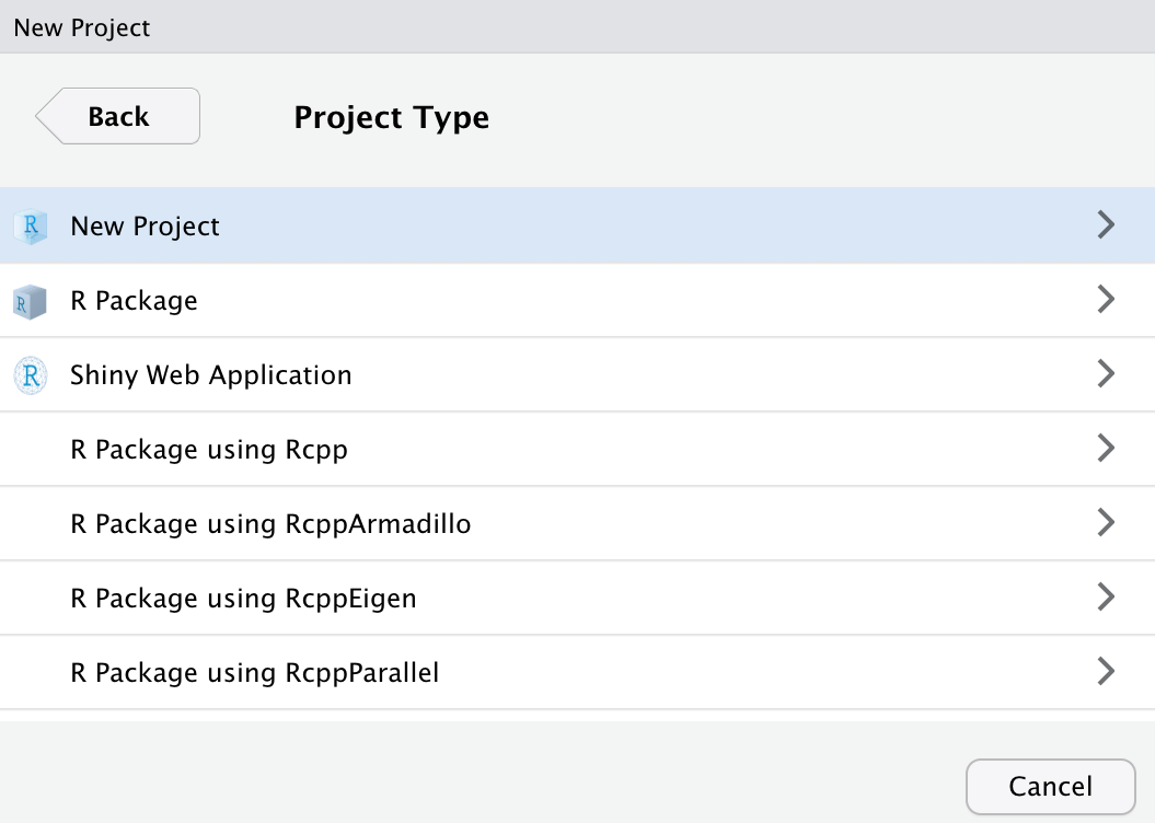
2. Select New Project as project type.
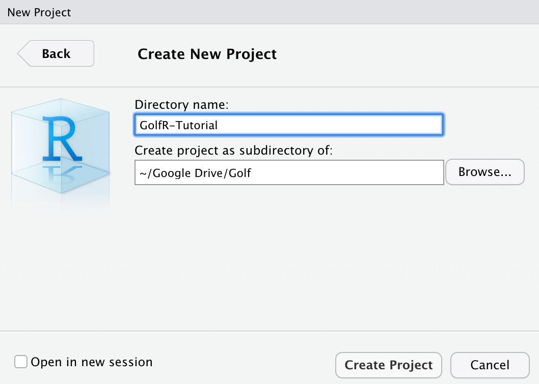
3. Name your new directory
4. Create new R Script…

If you’ve made it this far, get pumped. We’re about to get to the fun stuff.

STEP 4: Load the Data into R and Prep it for Analysis
Okay! We’re ready to start scripting in R.
A Note to Beginners
If you’ve never written any code before, that’s totally fine! A lot of the following will be foreign to you, but you should be able to just copy/paste these code chunks into your R-script (the top left pane of your R-Studio screen) and run it line by line to produce the same results. If you get errors, try unblocking yourself by Googling the errors or looking for solutions on a site like Stack Overflow.
I also highly recommend taking an “Intro to R” course like this one offered by Data Camp.
Let’s start by loading the packages that are going to help with the manipulation and visualization of our data. You can think of packages like libraries of specialized functions that help us do things we can’t do with R as it comes out of the box.
You can install them by copy/pasting the following code into your R script (top-left pane), and running in the terminal (low-left pane) by clicking “Run” (Mac: Cmd + Return, Windows: Ctrl + Enter).
# Let's do this in two steps.
# First, create a vector of the packages we'll need for this tutorial
packages <- c('tidyverse', 'janitor', 'corrplot', 'ggthemes', 'DT')
# Now, pass the vector you just created into the pkgs
# argument of the install.packages() function
install.packages(pkgs = packages)# We can load them one by one using the library function
library(tidyverse)
library(janitor)
library(corrplot)
library(ggthemes)
library(DT)# Or we can do it the fancy way. Learning the `apply` set of
# functions will save you a lot of time in R
lapply(X = packages, FUN = require, character.only = TRUE)You may get some warning messages, and if you run into trouble, the only packages we really need for this tutorial are tidyverse and janitor, so get rid of headaches if necessary.
When we created a new project, we created a directory to store all files associated with the project. Let’s go ahead and use the getwd() function to check where that working directory is on our machine.
# Check our current working directory
getwd()
## [1] "/Users/yourname/project_directory"Yours will likely look different, but the important thing to realize is that this location is where R will look for any data you’re looking to import. It’s also where it will write anything we export.
Now, let’s use the dir.create() function to create a subfolder where we’ll store our Foresight report data.
# Create a new folder within our working directory called "Data"
dir.create("Data")
A Note on Functions
If you ever have questions about the specific functions and the arguments they take, you can add a question mark before the function name and run it in your console to get the documentation. For instance, running ?read_csv() will tell us about that function.
Take your launch monitor data file and save it into the folder you just created. For your first run, I’d suggest just downloading the sample data I’ve provided so that if you run into trouble with running any of the following code, we can be sure it’s not a problem with your export.
We’re now going to read that dataset into R. Steps explained within the #commentary of the code.
# First, let's practice creating variables by making one for the
# path from the working directory to the data we just stored
file_name <- "Data/Foresight_Report_Numeric.csv"

# Next, we'll make use of the read_csv() function to pull in our dataset.
# You can see here that the read_csv() function is accepting the file_name
# object we just created.

# The first line of the Foresight report contains the name of the golfer
# and datetime of the launch monitor session.
report_details <- read_csv(file = file_name, col_names = FALSE, trim_ws = TRUE, n_max = 1)
Extract some metadata about the session that we’ll use later
# Some regex to extract the username and get datetime values
# We'll add these as columns back into our dataset later
username <- str_extract(report_details$X1, "(?<=: ).*(?= -)")
datetime <- as.POSIXct(str_extract(report_details$X1, "(?<= - ).*"), format = '%m/%e/%Y %I:%M %p', tz=Sys.timezone())
Now, let’s read in the variable names from our report.
# # In the Foresight reports I've seen, the names of the variables come in the second row.
# # We pull those in here by skipping the first row of our data
variables <- read_csv(file_name, skip = 1, col_names = FALSE, trim_ws = TRUE, n_max = 1)
Next, let’s pull in the full tablee and use our variables object to name the columns.
# We then pull in the actual data
raw_data <- read_csv(file_name, skip = 4, col_names = FALSE, trim_ws = TRUE)

# Change the column names of the raw data to our variable names
colnames(raw_data) <- variables
Let’s take a look at our dataset using the glimpse() function
# Take a look at our data
glimpse(raw_data)
## Rows: 66
## Columns: 25
## $ Club <chr> "Driver", "Driver", "Driver", "Driver", "Driver…
## $ Ball <chr> "Standard", "Standard", "Standard", "Standard",…
## $ `Ball Speed` <dbl> 157.9, 155.6, 153.1, 159.0, 158.0, 158.5, 155.9…
## $ `Launch Angle` <dbl> 17.3, 13.1, 17.0, 16.4, 16.0, 16.0, 17.6, 13.2,…
## $ `Side Angle` <dbl> 5.6, 2.7, 1.1, 3.0, 4.1, 3.9, 3.6, 1.6, 2.8, 4.…
## $ Backspin <dbl> 3074, 3669, 2474, 3114, 3223, 1123, 2573, 3218,…
## $ Sidespin <dbl> -67, -201, -26, -255, -87, -1275, -98, -211, -1…
## $ `Tilt Angle` <dbl> -1.2, -3.1, -0.6, -4.7, -1.5, -48.6, -2.2, -3.8…
## $ `Total Spin` <dbl> 3075, 3675, 2474, 3124, 3224, 1699, 2575, 3225,…
## $ Carry <dbl> 264.8, 250.6, 268.3, 265.9, 262.5, 257.1, 271.7…
## $ Total <dbl> 282.8, 267.2, 287.7, 282.9, 280.1, 283.0, 290.2…
## $ Offline <dbl> 24.1, 4.2, 4.0, 1.8, 15.6, -58.0, 12.2, -1.8, -…
## $ `Descent Angle` <dbl> 48.9, 45.9, 45.3, 48.3, 48.1, 31.9, 46.9, 43.5,…
## $ `Peak Height` <dbl> 52.8, 41.7, 46.6, 50.8, 49.7, 28.3, 50.3, 38.2,…
## $ `To Pin` <dbl> 95.7, 107.4, 86.9, 91.6, 96.0, 113.6, 85.3, 107…
## $ `Club Speed` <dbl> 109.1, 109.6, 108.7, 109.9, 110.3, 110.2, 108.8…
## $ Efficiency <dbl> 1.45, 1.42, 1.41, 1.45, 1.43, 1.44, 1.43, 1.39,…
## $ `Angle of Attack` <dbl> 6.8, 7.1, 8.2, 7.0, 6.7, 7.1, 7.8, 7.6, 7.2, 7.…
## $ `Club Path` <dbl> 5.3, 5.5, 4.4, 4.4, 5.5, 4.6, 4.8, 5.1, 4.1, 4.…
## $ `Face to Path` <chr> "--", "--", "--", "--", "--", "--", "--", "--",…
## $ Lie <chr> "--", "--", "--", "--", "--", "--", "--", "--",…
## $ Loft <chr> "--", "--", "--", "--", "--", "--", "--", "--",…
## $ `Closure Rate` <chr> "--", "--", "--", "--", "--", "--", "--", "--",…
## $ `Face Impact Lateral` <chr> "--", "--", "--", "--", "--", "--", "--", "--",…
## $ `Face Impact Vertical` <chr> "--", "--", "--", "--", "--", "--", "--", "--",…Here we get our first peak our data in its table format (technically it’s a tibble, but we won’t get into that here).
If you are using the sample data or followed the steps to export your own data, you should have a table with 25 variables that is roughly as many observations (rows) as balls hit during your session. I say “roughly” as many because if we look a little bit closer, there are some issues that may stand out.
tail(raw_data)## # A tibble: 6 × 25
## Club Ball `Ball Speed` `Launch Angle` `Side Angle` Backspin Sidespin
## <chr> <chr> <dbl> <dbl> <dbl> <dbl> <dbl>
## 1 3-Wood Standard 157. 13 3 2731 -812
## 2 3-Wood Standard 158. 12.5 4.2 3661 -320
## 3 3-Wood Standard 151 15.4 6 3068 201
## 4 3-Wood Standard 156. 14.2 6.7 3335 -310
## 5 Average <NA> 155. 12.8 4.3 3188 -335
## 6 Std. Dev. <NA> 4.4 2 1.7 695 449
## # … with 18 more variables: Tilt Angle <dbl>, Total Spin <dbl>, Carry <dbl>,
## # Total <dbl>, Offline <dbl>, Descent Angle <dbl>, Peak Height <dbl>,
## # To Pin <dbl>, Club Speed <dbl>, Efficiency <dbl>, Angle of Attack <dbl>,
## # Club Path <dbl>, Face to Path <chr>, Lie <chr>, Loft <chr>,
## # Closure Rate <chr>, Face Impact Lateral <chr>, Face Impact Vertical <chr>If you look closely you’ll there are a couple summary rows that give the average and standard deviations for each club hit during your session. That’s helpful if we’re just wanting to examine a .csv, but we’re going to go a bit deeper than that here, and if we want to look at summaries, we’ll create them on our own.
A Note on Data Prep
In addition to removing the Average and Std. Dev. summary rows, there are a few other things we need to do to get this dataset into shape. We could take those tasks one at a time as we encounter them, but that can be inefficient, if for no other reason than you end up with a bunch of intermediate tables called temp_data_1, temp_data_2, and so on.
Instead, we can use the %>% (called a pipe operator), that allows us to take the output from one step and perform additional manipulation in the next. You can think of it as the “and then” operator because it’s telling R, “take the output from the last step, and then do X”. I’ll show what I mean.
In this next chunk of code, I’m going to create a new table called clean_data. The first thing I’m going to feed into clean_data will be our raw_data table. I’m then going to perform three separate transformations before returning our new clean_data table.
# Create new table called clean_data.
# Start with raw_data table
# and then change the casing of the column names
# and remove any rows that are blank or have 'Average' or 'Std. Dev.'
clean_data <- raw_data %>%
  clean_names(case = "snake") %>%
  # Basically reads "don't keep any rows where the value for the club variable is one of these
  filter(! club %in% c('Average', 'Std. Dev.', NA)) %>%
  # Coerce all our variables, except for "club" and "ball" to numerics.
  # This ensures that for any values where we didn't get a reading,
  # we get a NA value rather than the '--' that comes standard in the Foresight report
  mutate_at(vars(-club, -ball), as.numeric)
There’s one more step we should probably take now before we begin our analysis. Let’s look at the values for a variable like ‘offline’. Note, putting a $ after the name of your table allows you to access a specific variable
# This will return the values from the 'offline' column of the 'clean_data' table
clean_data$offline
## [1] 24.1 4.2 4.0 1.8 15.6 -58.0 12.2 -1.8 -53.4 30.7 -8.3 -76.4
## [13] 39.1 -5.1 39.5 -9.3 18.6 5.3 -14.1 25.8 -43.3 -4.6 14.0 -8.1
## [25] -0.4 42.4 -51.6 -44.0 29.6 41.3 20.4 -45.2 -17.0 22.4 22.7 -14.2
## [37] -7.0 11.0 24.0 -46.7 21.9 -13.3 15.6 57.1 7.0 29.3 -33.5 3.7
## [49] -20.9 26.1 -12.0 -3.9 -17.5 1.7 25.2 -3.4 -1.0 -27.8 6.1 37.8
## [61] 17.8If you have any kind of a normal shot pattern, some of these values will be negative and some will be positive. The negative values are shots that were missed to the left, the positive values are shots that were missed to the right. When we begin exploring our data, it would be nice to be able to do things like a simple count of the number of shots that were missed left, without having to do additional manipulation.
We have a similar issue with the variables for side_angle, sidespin, tilt_angle, angle_of_attack, and club_path. If you have a GCQuad, you may have to do similar transforms for face_to_path, lie, closure_rate, face_impact_lateral and face_impact_vertical. If you have an example dataset with those variables, shoot it my way and I’ll add some code to the repo.
Anyway, let’s make use of the mutate() function to create new variables for these directional categories. If you’d like to know more about the case_when() function, check out this tutorial.
Additionally, we’re going to add back in our values for username and datetime so that if we build a larger dataset of multiple sessions, or multiple people, we’ll have an easy way to compare.
A Note to Lefties
I haven’t verified that these transformations are all correct for left-handed golfers, so if you see something I missed or have left-handed Foresight data you want to share, let me know.
transformed_data <- clean_data %>%
  mutate(side_angle_dir = case_when(side_angle > 0 ~ 'Right', side_angle < 0 ~ 'Left',
                                    side_angle == 0 ~ 'Center', TRUE ~ 'No Reading'),
         sidespin_dir = case_when(sidespin > 0 ~ 'Right', sidespin < 0 ~ 'Left',
                                  sidespin == 0 ~ 'No Sidespin', TRUE ~ 'No Reading'),
         tilt_angle_dir = case_when(tilt_angle > 0 ~ 'Right', tilt_angle < 0 ~ 'Left',
                                    tilt_angle == 0 ~ 'No Tilt Angle', TRUE ~ 'No Reading'),
         offline_dir = case_when(offline > 0 ~ 'Right', offline < 0 ~ 'Left',
                                 offline == 0 ~ 'Center', TRUE ~ 'No Reading'),
         angle_of_attack_dir = case_when(angle_of_attack > 0 ~ 'Up', angle_of_attack < 0 ~ 'Down',
                                         angle_of_attack == 0 ~ 'Neutral AoA', TRUE ~ 'No Reading'),
         club_path_dir = case_when(club_path > 0 ~ 'In-to-Out', club_path < 0 ~ 'Out-to-In',
                                   club_path == 0 ~ 'Neutral Path', TRUE ~ 'No Reading'),
         face_to_path_dir = case_when(as.numeric(face_to_path) > 0 ~ 'In-to-Out', as.numeric(face_to_path)  < 0 ~ 'Out-to-In',
                                   as.numeric(face_to_path)  == 0 ~ 'Neutral Path', FALSE ~ 'No Reading'),
         date_time = datetime,
         username = username
         )
Okay! We now have a clean dataset that’s ready for analysis. Let’s take a look!
head(transformed_data)## # A tibble: 6 × 34
## club ball ball_speed launch_angle side_angle backspin sidespin tilt_angle
## <chr> <chr> <dbl> <dbl> <dbl> <dbl> <dbl> <dbl>
## 1 Driver Standa… 158. 17.3 5.6 3074 -67 -1.2
## 2 Driver Standa… 156. 13.1 2.7 3669 -201 -3.1
## 3 Driver Standa… 153. 17 1.1 2474 -26 -0.6
## 4 Driver Standa… 159 16.4 3 3114 -255 -4.7
## 5 Driver Standa… 158 16 4.1 3223 -87 -1.5
## 6 Driver Standa… 158. 16 3.9 1123 -1275 -48.6
## # … with 26 more variables: total_spin <dbl>, carry <dbl>, total <dbl>,
## # offline <dbl>, descent_angle <dbl>, peak_height <dbl>, to_pin <dbl>,
## # club_speed <dbl>, efficiency <dbl>, angle_of_attack <dbl>, club_path <dbl>,
## # face_to_path <dbl>, lie <dbl>, loft <dbl>, closure_rate <dbl>,
## # face_impact_lateral <dbl>, face_impact_vertical <dbl>,
## # side_angle_dir <chr>, sidespin_dir <chr>, tilt_angle_dir <chr>,
## # offline_dir <chr>, angle_of_attack_dir <chr>, club_path_dir <chr>, …datatable(transformed_data, rownames = FALSE, filter = "top", options = list(pageLength = 5))